What’s Involved In Running A Dovetail^® HiChIP Assay?
(Part 2)

You’ve generated your HiChIP libraries, had them sequenced, and are now wondering what to do with your data. Don’t worry, we will walk you through the process step by step and by the end of this article, you will have a strategy for making sense of your HiChIP data and be well on your way to making new discoveries!  

Stage 0: Install the Tools

The HiChIP informatics workflow relies on a number of open-source program packages to enable the conversion of sequence data to biological insights. To make use of these packages, you will have to spend a little time configuring your bioinformatics environment. But don’t worry, we provide detailed instructions on how to complete this here.

Step 1: Alignment and Pairs Generation

Once the tools are installed and all relevant files have been gathered, you will perform the following actions:

1. Align your HiChIP *.fastq file to your genome reference file
2. Parse and sort the valid ligation events
3. Remove any PCR duplicates

More details on how to complete this step are provided here. The output stats file generated during this step will be used in the next step to QC your library.

Step 2: Library QC

When assessing data quality, we are interested in confirming:

1. The amount of long-range information captured by the library
2. The degree of enrichment achieved by the chromatin immunoprecipitation (ChIP) step

Within the stats file generated in Step 1, you will find metrics describing the long-range quality of the library, so you are already halfway there.

Tip: for mammalian samples, we consider them acceptable if the “mapped no-dup cis read pairs > 1kb” stat is greater than 20% of the total mapped no-dup pairs.

It is useful to note that HiChIP data is composed of primary peaks that represent direct protein binding, and secondary peaks that result from interactions occurring in 3D chromatin space. For the purpose of assessing ChIP success, we want to focus on primary peaks in our HiChIP data.

In a successful ChIP experiment, we expect our read-pairs coverage distribution to be biased towards our primary peaks given that these are the targets of enrichment. Therefore, to assess the extent of enrichment, we can compare the depth of our HiChIP reads at primary peaks to the expected number of reads if the read-pairs were evenly distributed across the genome. This computed observed/expected coverage ratio provides a measure of enrichment.

A visual check is also useful: plotting normalized sequence coverage around our primary peaks offers a profile of ChIP enrichment.

Tip: the script plot_chip_enrichment.py identifies ChIP peak regions, sets 1 kb windows up- and down-stream of the peak centers, calculates read coverage within these windows, and then plots the global fold coverage change.

The figure below is an example of a passing QC plot. Note the significantly higher coverage centered over the peak centers compared to the outlying area. The height and shape of this plot will depend on the antibody used, however.https://dovetailgenomics.com/wp-content/uploads/2021/04/hichip-blog-2_coverage.png

At this point, you should be confident that your data is of high-quality and be ready to move onto visualizing your HiChIP data for final analysis!

Step 3: Data Analysis & Visualization

This is where it starts to get fun. As with all Hi-C datatypes, the next step is to generate your contact matrix. This enables proximal ligations produced in the HiChIP assay to be visualized and is an input for the subsequent steps. You have two options for viewing your data: Juicebox (as part of Juicer tools) or HiGlass.

Keep in mind, different from standard Hi-C data, HiChIP data identifies significant interactions between your protein of interest and the surrounding genome. As such, HiChIP data highlights chromatin “loops” that are anchored at a protein binding site. So, next up in our analysis path is calling and visualizing those loops.

There are a number of different tools that can be used for this, some of which we call out in the table below:

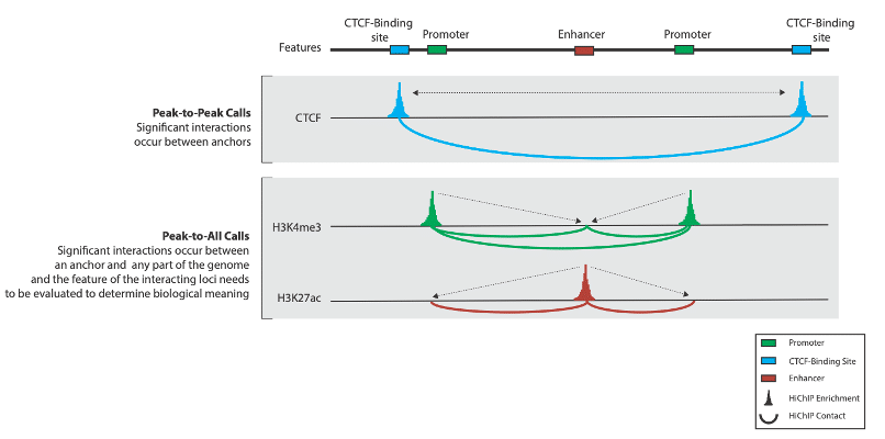
*What are “interaction types,” you may be wondering? There are three main interactions that help describe the loops we’ll be calling in a bit: peak-to-peak, peak-to-all, and all-to-all. We describe each of these in the FAQs section at the end.

In our step-by-step guide, we take you through an example workflow using FitHiChIP that enables you to plot your HiChIP data and visualize the chromatin loops. After some editing in Adobe Illustrator (or another PDF editor), you should end up with something similar to the following figure:https://dovetailgenomics.com/wp-content/uploads/2021/04/hichip-blog_img2.pngAnd voilà! We are left with a beautiful figure that reflects interactions between our protein of interest and the DNA surrounding it. Now, determining what it all means is your job, and we can’t wait to read all about it in future publications!

Still have questions? For step-by-step instructions, please check out our complete HiChIP documentation that will walk you through the concepts described above in detail.

FAQs

1. What are chromatin loops in the context of HiChIP and what do they mean? Can you give me some examples?

The term chromatin loop is used here somewhat loosely and defined as significant interactions between a protein-anchor and somewhere else in the genome. The biological interpretation of these depends on the protein of interest. Note that a stricter definition of chromatin loops exists, and this class is exclusively dependent upon CTCF and cohesin. It is also worth mentioning one additional class: H3K27ac and H3Kme3 highlight regions that interact with the enhancer or promoter, respectively.

2. What are the significant types of interactions you mentioned before? 

There are two main types of interactions that we’re typically interested in:

• • • Peak-to-peak are interactions between primary sites of protein binding. A good example of these types of interactions is found in HiChIP datasets anchored on CTCF.
    • Peak-to-all involve interactions between the primary peaks and other regions in the surrounding genome, regardless of whether those regions correspond to another anchor or not. Examples of these types of interactions occur in datasets anchored at H3K27ac, H3Kme3, and PolII.
    • A third type, all-to-all, are typically for non-targeted Hi-C data, so we generally ignore these.

The figure below illustrates the difference between the two that we are most interested in.

3. What is the recommended bin size for loop calling?

You should bin between 1-10 kb (most HiChIP analyses are binned between 2.5-5 kb).

Your bin size will depend on the protein you are targeting. Proteins with larger footprints (i.e. PolII) will benefit from a larger bin size, while those with smaller footprints (i.e. CTCF) should have a smaller bin. Additionally, larger bin sizes should be considered when you have fewer reads per interaction (just be conscious of not making your bins so large that you capture multiple anchors in one bin). We recommend trying to call significant interactions at a few different bin sizes and filtering out the unique entries.

4. What if I don’t have a *.bed file of ChIP-seq anchors, or can’t find one that is representative of my sample/antibody?

We have a guide for that! Check out calling 1D peaks with HiChIP data using MACS2.